Home >>STATISTICS, Section 1, dispersion 3
first principles |
Variance - Var(X)
Variance is a measure of dispersion(the spread of data).
The variance of a random variable X is given by:

where,
xr is any value of the random variable X
μ is the mean value of X
n is the number of values of X
Σ means the sum of all values in the brackets
The variance can also be expressed in terms of the standard deviation σ :
![]()
Standard Deviation - symbol σ (sigma)
Like variance, standard deviation is also a measure of dispersion.
From the equations above, it follows that :

and,

Example
Calculate the variance and standard deviation of the following data set of 10 numbers(n = 10). Answer to 3 significant figs.
1, 1, 3, 4, 4, 5, 7, 7, 9, 10
the mean, 
![]() = (1 - 5.1) + (1 - 5.1 ) + (3 - 5.1) + (4 - 5.1) + (4 - 5.1) + ( 5 - 5.1) + (7 - 5.1 ) + (7 - 5.1 ) + ( 9 - 5.1) + (10 - 5.1)
= (1 - 5.1) + (1 - 5.1 ) + (3 - 5.1) + (4 - 5.1) + (4 - 5.1) + ( 5 - 5.1) + (7 - 5.1 ) + (7 - 5.1 ) + ( 9 - 5.1) + (10 - 5.1)
= (-4.1) + (-4.1) + (-2.1) + (-1.1) + (-1.1) + (-0.1) + (1.9) + (1.9) + (3.9) + (4.9)
![]() = 16.81 + 16.81 + 4.41 + 1.21 + 1.21 + 0.01 + 3.61 + 3.61 + 15.21 + 24.01
= 16.81 + 16.81 + 4.41 + 1.21 + 1.21 + 0.01 + 3.61 + 3.61 + 15.21 + 24.01
= 86.9

answer: variance(σ2) is 8.69 , standard deviation(σ) is √8.69, that is 2.94788 or 2.95 (3sf)
Variance and Standard Deviation for Grouped Data
Recalling that for grouped data, the estimated mean is given by:

The definition of variance(σ2) for grouped data is :

where x is the mid-value for each group of data.
Example
The grouped data in the table represents the exam marks(m) and their frequency(f) for 100 students.
Estimate the variance and standard deviation to 2 decimal places.
m |
0≤m<20 |
20≤m<40 |
40≤m<60 |
60≤m<80 |
80≤m<100 |
f |
3 |
19 |
51 |
22 |
5 |
m |
mid-interval value x |
f |
fx |
x2 |
fx2 |
0≤m<20 |
10 |
3 |
30 |
100 |
300 |
20≤m<40 |
30 |
19 |
570 |
900 |
17100 |
40≤m<60 |
50 |
51 |
2550 |
2500 |
127500 |
60≤m<80 |
70 |
22 |
1540 |
4900 |
107800 |
80≤m<100 |
90 |
5 |
450 |
8100 |
40500 |
sum Σ |
100 |
5140 |
293200 |
The estimated mean is given by :

The variance is given by :


answer: variance is 290.04 , standard deviation is 17.03 ( √290.04 )
Skewness
Skewness is the degree to which a normal distribution is distorted.
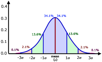
A Normal (or Gaussian) Distribution is a symmetrical curve, with a central maximum.
The mean, mode and median all occur at one point along the x-axis, corresponding to the central maximum.

where SD stands for Standard Deviation σ(sigma):
| 68.2% of values are 1 SD from the mean 95.4% of values are 2 SD from the mean 99.6% of values are 3 SD from the mean |
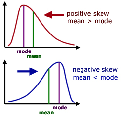
When a distribution is skewed the curve is no longer symmetrical.
The central maximum is moved either to the right or the left.

A positive skew is when the right tail is longer. The central maximum is to the left of the figure and the mean is greater than the mode.
A negative skew is when the left tail is longer. The central maximum is to the right of the figure and the mean is less than the mode.
Skewness can be simply measured using either :
The Pearson Mode Coefficient of skewness

The Pearson Median Coefficient of skewness

The resulting number obtained from each method is the same.
Another method of measuring skewness concerns quartiles (Q1 Q2 Q3 ).

Outliers
These are observations that appear to deviate markedly from other members of the sample in which they occur.

For computing 'line of best fit' and other statistical operations, good practice is to discard outliers before processing data.
[ About ] [ FAQ ] [ Links ] [ Terms & Conditions ] [ Privacy ] [ Site Map ] [ Contact ]
